Quick Start

This page walks through the most common workflow: load an instrument template, tweak parameters, run a simulation, and inspect the result.

1. Create a TipTop object

Load a built-in instrument template by name:

from tiptop_ipy import TipTop

tt = TipTop("ERIS")

You can also load from a custom .ini file:

tt = TipTop(ini_file="my_custom_config.ini")

Or start from blank defaults:

tt = TipTop()

2. Inspect the configuration

In Jupyter, simply evaluate the object to see an HTML table of all parameters:

tt  # renders rich HTML table in Jupyter

Access a whole section:

tt["atmosphere"]
# {'Wavelength': 5e-07, 'Seeing': 0.8, 'L0': 25.0, ...}

Access a single parameter with tuple indexing:

tt["atmosphere", "Seeing"]
# 0.8

3. Modify parameters

tt["atmosphere", "Seeing"] = 0.6
tt["telescope", "ZenithAngle"] = 15.0

Check what you’ve changed:

tt.diff()
# {'atmosphere': {'Seeing': (0.8, 0.6)},
#  'telescope': {'ZenithAngle': (30.0, 15.0)}}

Reset to the original template values at any time:

tt.reset()

Setting wavelengths

The wavelengths property works in microns by default, or accepts any astropy.units.Quantity:

import astropy.units as u

tt.wavelengths                     # current value as Quantity in µm
# <Quantity [1.65] um>

tt.wavelengths = [1.2, 1.65, 2.2]          # plain floats → microns
tt.wavelengths = [500, 700] * u.nm          # nanometres
tt.wavelengths = 16500 * u.AA               # Angstrom

The internal config (sources_science.Wavelength) is always stored in metres, but you never need to worry about that.

Setting off-axis positions

Use add_off_axis_positions to specify where on the sky the PSFs should be generated, using Cartesian (x, y) coordinates:

# On-axis + 5" offset in x and y (plain floats → arcsec)
tt.add_off_axis_positions([(0, 0), (5, 5)])

# With explicit units
tt.add_off_axis_positions([(0, 0), (5 * u.arcmin, 0 * u.arcsec)])

Read back the current positions:

x, y = tt.positions    # Quantity arrays in arcsec
# (<Quantity [0., 5.] arcsec>, <Quantity [0., 5.] arcsec>)

Under the hood this converts to sources_science.Zenith (radial distance) and sources_science.Azimuth (angle from the x-axis in degrees).

4. Validate the configuration

Check for errors before sending to the server:

issues = tt.validate()
for issue in issues:
    print(issue)

5. Run the simulation

result = tt.generate_psf()

This sends the configuration to the TIPTOP server and returns a TipTopResult object. The call validates the configuration first and will raise ValueError if there are errors.

6. Work with the result

# Quick plot (works in Jupyter)
result.plot()

# Access the PSF data as a numpy array
result.psf          # 2D or 3D array
result.psf.shape    # e.g. (1, 256, 256)

# Strehl ratio and FWHM
result.strehl       # e.g. array([0.891])
result.fwhm         # e.g. array([44.1])  (mas)

# Coordinates of each PSF position
result.x  # arcsec
result.y  # arcsec

# Get the PSF nearest to a sky position
psf = result.nearest_psf(x=5.0, y=3.0)

# Multi-wavelength: access each cube
result.n_wavelengths  # e.g. 3
result.psf_cube(0)    # first wavelength
result.psf_cube(1)    # second wavelength

# Save to FITS
result.writeto("my_psf.fits", overwrite=True)

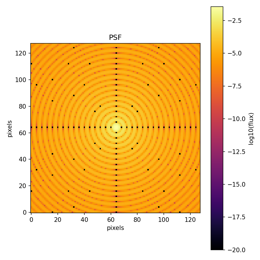
Example: plotting a synthetic PSF

The TipTopResult.plot() method produces a log-scaled PSF image. Below is a demonstration using a synthetic Airy-like PSF (no server connection required):

import numpy as np
import matplotlib.pyplot as plt
from astropy.io import fits
from tiptop_ipy.result import TipTopResult

# Generate a synthetic Airy-like PSF
size = 128
y, x = np.mgrid[-size//2:size//2, -size//2:size//2]
r = np.sqrt(x**2 + y**2).astype(float)
r[r == 0] = 1e-10
psf = (np.sin(np.pi * r / 4) / (np.pi * r / 4))**2
psf /= psf.sum()

# Build a mock FITS HDUList matching TIPTOP server format
primary = fits.PrimaryHDU()
hdr = fits.Header()
hdr["CONTENT"] = "PSF CUBE"
hdr["WL_NM"] = 1650
hdr["PIX_MAS"] = 14
hdr["CCX0000"] = 0.0
hdr["CCY0000"] = 0.0
hdr["SR0000"] = 0.85
hdr["FWHM0000"] = 50.0
cube = fits.ImageHDU(data=psf[np.newaxis, :, :].astype(np.float32), header=hdr)

ol_hdr = fits.Header(); ol_hdr["CONTENT"] = "OPEN-LOOP PSF"
ol = fits.ImageHDU(data=np.random.rand(size, size).astype(np.float32), header=ol_hdr)

dl_hdr = fits.Header(); dl_hdr["CONTENT"] = "DIFFRACTION LIMITED PSF"
dl = fits.ImageHDU(data=psf.astype(np.float32), header=dl_hdr)

pr_hdr = fits.Header(); pr_hdr["CONTENT"] = "Final PSFs profiles"
pr = fits.ImageHDU(data=np.random.rand(2, 1, size//2).astype(np.float32), header=pr_hdr)

hdulist = fits.HDUList([primary, cube, ol, dl, pr])
result = TipTopResult(hdulist)

# Use the built-in plot method
fig, ax = result.plot()
plt.show()

7. Save and reload configs

# Save the current configuration
tt.save("my_config.ini")

# Load it back later
tt2 = TipTop(ini_file="my_config.ini")